
HLOOKUP is one of the basic functions in Excel that is used very commonly today. In this article, I will help you better understand the function and how to use it!
1. Learn about the Excel HLOOKUP function
The Excel HLOOKUP function finds and retrieves a value from data in a horizontal table. The “H” in HLOOKUP stands for “horizontal” and lookup values should appear in the first row of the table, moving horizontally to the right.
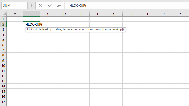
Syntax:
=HLOOKUP (lookup_value, table_array, row_index, [range_lookup])
Where the function arguments are as follows:
lookup_value: The value you want to look up, in the first row of the table
table_array: The table or array from which to retrieve data.
row_index: The row number in the supplied table from which you want to retrieve data.
range_lookup: [optional] Use TRUE or 1 for an approximate match and FALSE or 0 for an exact match.
- TRUE: if the function cann’t find an exact match, it uses an approximate match.
- FALSE: if the function cann’t find an exact match, it will return an error.
2. Excel HLOOKUP Function Examples
Example 1: Student ranking – exact match
In the example below, we need to rank the students in Table 1 (B3:D8) with the data in Table 2 (B11:F12).
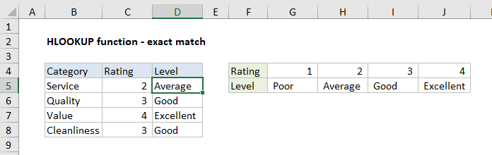
In cell D5, the HLOOKUP formula, copied down, is:
=HLOOKUP(C5,$G$4:$J$5,2,FALSE) // exact match
The HLOOKUP function will look up the score in cell C5 in Table 2 from left to right. When it finds a value equal to lookup_value, it returns the corresponding rating in row 2.
Example 2: Student ranking – approximate match
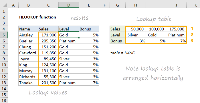
In the screen above, the goal is to look up the correct Level and Bonus for the sales amounts in C5:C13. To lookup Level, the formula in cell D5 is:
=HLOOKUP(C5,$H$4:$J$6,2,1) // get level
For each amount in C5:C13, the goal is to find the best match, not an exact match.
To lookup Bonus, the formula in cell D5, is:
=HLOOKUP(C5,$H$4:$J$6,3,1) // get bonus
Note again, range_lookup is set to TRUE or 1 to require approximate match.
3. Common errors when using the Excel HLOOKUP function
If you get an error from Excel’s Hlookup function, it may be due to one of the following errors:
Error #N/A
This is a common error if the HLOOKUP function cannot find a match for the supplied lookup_value.
The cause of this usually depends on the value of [range_lookup] provided:
- if [Range_lookup] = TRUE (or empty) the #N/A error occurs because the smallest value in the lookup row is greater than the supplied lookup_value.
- if [Range_lookup] = FALSE, the #N/A error occurs because an exact match to lookup_value was not found in the lookup row.
Error #REF!
Error #REF! usually occurs if the row_index_num argument is greater than the number of rows in the supplied table_array.
Error #VALUE!
This is a common error due to 2 reasons:
First: Since the row_index_num argument is < 1 or not a number.
Second: Because the [range_lookup] argument is not recognized as TRUE or FALSE.
Above, I showed you how to use the Excel HLOOKUP function. Hopefully through this article you have understood the syntax and usage of this function so that you can apply it in practice.